
Supervised Speech Enhancement with Self-Attention
Published:
About This Article
TL;DR: This article introduces a Deep Generative Speech Enhancement model that utilizes a hybrid architecture combining the U-Net Architecture and Transformers. The model, CleanUNet, operates on raw waveforms and uses causal convolutions for real-time applications. It refines speech using a multi-resolution STFT loss, targeting both high and low frequencies. The model was trained on the VoiceBank + Demand dataset and outperforms other state-of-the-art models in benchmark tests. Detailed sections include model architecture, training setup, loss functions, and evaluation.
The model is trained in a supervized manner to remove various types of noise from audio signals, enhancing the clarity and quality of speech. We have tested the model on several noise conditions, demonstrating its effectiveness across different environments.
You can find the implementation from scratch using PyTorch Here.
Before diving right in, it would be a great idea to check out this awesome piece on Transformers and The Attention Mechanism written by one of the most insightful AI bloggers, Lilian Weng. Since these concepts form the backbone of the architecture used in the model we're using, getting familiar with them will make it a breeze to follow along with the rest of the article.
Also, if you’re not familiar with Convolutions or Convolution Neural Networks (CNNs) in general, here is a great resource with good visualizations that explains how CNNs work.
Audio Samples
Introduction
Speech enhancement is crucial area of research in the field of signal processing, with applications in improving the quality, clarity and intelligibility of speech signals in various environments. It involves processes to reduce background noise, remove unwanted acoustic artifacts, and amplify desired speech components. This technology finds applications in diverse fields such as telecommunications, hearing aids, speech recognition systems, audio/video conferencing, and broadcast media. [1] [2]
Traditional signal processing methods, such as spectral subtraction [3] and Wiener filtering [4], are required to produce an estimate of noise spectra and then the clean speech given the additive noise assumption. These methods work well with stationary noise process, but may not generalize well to nonstationary or structured noise types such as dogs barking, baby crying, or traffic horn. Recent advances in deep learning have led to significant improvements in speech enhancement performance. However, there is still much to explore in terms of model architectures and training approaches.
The model in question is based on a supervised approach described in the paper "Speech Denoising in the Waveform Domain with Self-Attention" by Kong et al. This method, called CleanUNet, operates directly on raw waveforms and leverages self-attention mechanisms to refine bottleneck representations in the U-Net network. [5]
The primary goal of the CleanUNet model is to effectively remove background noise from recorded speech while maintaining the perceptual quality and intelligibility of the speech signals. This model addresses the limitations of traditional signal processing methods by utilizing the increased computational power of deep neural networks to achieve state-of-the-art results in speech enhancement.
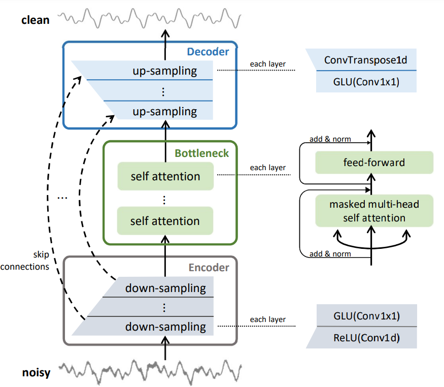
The architecture of CleanUNet consists of three main components: an encoder, a bottleneck with self-attention blocks, and a decoder. The encoder compresses the input waveform into a lowerdimensional representation -- an embedding, which is then refined by the self-attention blocks in the bottleneck. Finally, the decoder reconstructs the denoised waveform from the refined representation. The model uses causal convolutions to ensure low-latency processing, making CleanUNet suitable for real-time applications.
The following sections will cover the model's architecture, the training supervision strategies, and the loss functions used to optimize its performance.
Furthermore the model will be benchmarked on the VoiceBank + Demand dataset [6] using various objective metrics (e.g. PESQ [7]). This evaluation will include a comparison with other state-of-theart models to demonstrate how the model outperforms them on various benchmarks.
The Model's Architecture
Problem Setting
The end goal is to have a model that can denoise speech collected from a single channel microphone (mono audio). The model is causal for online streaming applications. A causal model only uses past and present information to make predictions, never future information. In the context of audio processing, this means the model only uses audio samples up to the current time to process or generate output. More formally, let $\mathbf{x}_\text{noisy} \in \mathbb{R}^T$ be the observed noisy speech waveform of length of length $T$. We assume the noisy speech is a mixture of clean speech $\mathbf{x}$ and background noise $\mathbf{x}_\text{noise}$ of the same lenght: $\mathbf{x}_\text{noisy} = \mathbf{x} + \mathbf{x}_\text{noise}$. The goal is to obtain a denoiser function $f$ such that:- $\hat{\mathbf{x}} = f(\mathbf{x}_\text{noisy}) \approx \mathbf{x}$
- $f$ is causal: the $t$-th element of the output $\hat{\mathbf{x}_t}$ is only a function of the previous observation $\mathbf{x}_\text{1:t}$
The U-Net Architecture
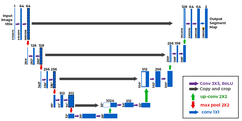
The backbone architecture of the model is the U-Net architecture [8] [9].U-Net was introduced in the paper "U-Net: Convolutional Networks for Biomedical Image Segmentation. This architecture was primarily developed to tackle the issue of limited annotated data in the medical field, allowing for effective use of smaller datasets while maintaining both speed and accuracy.
U-Net's structure is distinctive, comprising two main components: a contracting path and an expansive path. The contracting path, or encoder, captures contextual information and reduces the spatial resolution of the input. Conversely, the expansive path, or decoder, reconstructs the data by upsampling and integrates information from the contracting path through skip connections to produce a segmentation map.
The Encoder and Decoder
Encoder
The encoder has $D$ layers, where $D$ is the depth of the encoder. Each encoder layer is composed of a strided 1-d convolution (one dimensional Convolution, Conv1d) followed by the rectified linear unit (ReLU) and a 1x1 convolution (Conv1×1) followed by the gated linear unit (GLU).
The Rectified Linear Unit (ReLU) function is one of the most commonly used activation functions in neural networks. Its primary purpose is to introduce non-linearity into the model while maintaining computational efficiency. The ReLU function is defined as follows: $$ \text{ReLU}(\mathbf{x}) = \max(0, \mathbf{x}) $$ The Gated Linear Unit (GLU) is an activation function that combines two linear transformations and a sigmoid activation function to modulate the input. The GLU function can be defined as follows: $$ \text{GLU}(\mathbf{x}) = (\mathbf{x} \cdot W_1 + b_1) \odot \sigma(\mathbf{x} \cdot W_2 + b_2) $$ where:
- $W_1$ and $W_2$ are weight matrices.
- $b_1$ and $b_2$ are bias vectors.
- $\sigma$ is the sigmoid activation function.
- $\odot$ denotes element-wise multiplication.
In causal convolutions, each output value depends only on the current and previous input values, not on future values. This is achieved by ensuring that the convolutional kernel only interacts with the past and present values, adhering to the causality constraint.
A 1-d convolution operation involves sliding a filter (or kernel) over a one-dimensional input sequence, performing element-wise multiplication, and summing the results to produce an output sequence.
Formally, for a 1-d causal convolution with kernel $K$ and input $\mathbf{x}$, the output $y$ at time step $t$ is: $$ y(t) = \displaystyle\sum_{i=0}^\text{k-1}\mathbf{x}(t-i) K(i),$$ where $k$ is the kernel size and $K(i)$ the kernel weights at position $i$. $\mathbf{x}(t-i)$ refers to the input at time $(t-i)$, ensuring that future values are not included in the computation. To maintain the length of the output sequence equal to the input sequence length, causal convolutions use zero-padding on the left side of the input sequence.
Decoder
The decoder has $D$ decoder layers, same as the encoder. Each decoder layer is paired with the corresponding encoder layer in the reversed order; for instance, the last decoder layer is paired with the first encoder layer. Each pair of encoder and decoder layers are connected via a skip connection. For each downsampling step, the output feature maps are saved. When the network reaches the corresponding upsampling step in the expansive path, these saved feature maps are concatenated with the upsampled feature maps. This concatenation merges high-resolution information from the encoder with the low-resolution feature maps being refined in the decoder. Each decoder layer is composed of a Conv1×1 followed by GLU and a transposed 1-d convolution (ConvTranspose1d).
The transposed convolution increases the size of the input sequence by inserting zeros between elements and then applying a convolution-like operation with a learnable kernel. The ConvTranspose1d in each decoder layer is causal and has the same hyperparameters as the Conv1d in the paired encoder layer, except that the number of input and output channels are reversed.
For a 1-d transposed convolution with a causal constraint, the operation involves spreading the input sequence and applying the kernel, while respecting the causality constraint. The result is an upsampled sequence.
More formally, Given an input sequence $\mathbf{x}$ of length $L$ and a kernel $k$ of length $K$, the causal 1-d transposed convolution can be represented as: $$ y(t) = \sum_{i=0}^{\min(t, L-1)} x(i) \cdot k(t - i) $$
The Bottleneck
To refine the bottleneck, we use masked self-attention to enhance the model's ability to capture long-range dependencies in the speech signal, which helps in distinguishing between speech and noise.Masked self-attention is a variant where a mask is applied to ensure that the model does not attend to future time steps adhering to the causality constraint necessary for real-time processing.
The mask is an upper triangular matrix that masks out the future time steps (i.e., sets their attention scores to negative infinity so that the SoftMax function gives them zero weight). The modified attention mechanism can be expressed as: $$\text{MaskedAttention(K,Q,V)} = \text{Softmax}\left(\frac{QK^T + M}{\sqrt{d_k}}\right) \cdot V$$ Where $M$ is the mask matrix, $M_\text{ij} = -\infty$ if $i \gt j$ and $M_\text{ij} = 0$ otherwise.
The bottleneck is composed of $N$ self-attention blocks. Each self-attention block is composed of a multihead self-attention layer and a position-wise fully connected layer. The position-wise fully connected layer applies a fully connected neural network independently to each position (or time step) of the input sequence.
Unlike traditional fully connected layers that connect all neurons across different positions, the position-wise layer operates on each position separately, allowing the model to process information locally at each time step while maintaining the sequence's overall structure.
The Loss Function
The loss function quantifies the error or difference between the generated speech and the actual clean speech, guiding the learning process during training.A simple loss function would be the $l_1$ loss on waveform, the first order norm of the difference between the clean speech $x$ and the generated speech $\hat{\mathbf{x}} = f(\mathbf{x_\text{noisy}})$, formally $ \lVert \mathbf{x} - \hat{\mathbf{x}} \rVert_1 $. With the model trained with $l_1$ loss, the silence part of the generated audio is clean, but the high frequency bands are not accurate.
Another loss function that could be defined is an STFT loss between clean speech and the denoised speech.
Let $s(\mathbf{x}, \theta) = \vert STFT(\mathbf{x}) \vert$ be the magnitude of the linear-scale spectrogram of $\mathbf{x}$, where $\theta$ represents the hyperparameters of the STFT including the window length and hop size (the amount of overlap between consecutive windows or frames).
The STFT loss [10] is defined as $$ \mathrm{M\text{-}STFT}(\mathbf{x},\hat{\mathbf{x}}) = \sum_{i=1}^m \left( \frac{\|s(\mathbf{x};\theta_i)-s(\hat{\mathbf{x}};\theta_i)\|_F}{\|s(\mathbf{x};\theta_i)\|_F} \right. + \left. \frac{1}{T} {\left\|\log \frac{s(\mathbf{x};\theta_i)}{s(\hat{\mathbf{x}};\theta_i)}\right\|_1} \right) $$ Where $m$ is the number of resolutions and $\theta_i$ is the STFT parameter for each resolution.
This model trained on the STFT loss alone leads to generating low-frequency noises on the silent part of the denoised speech.
As a result, a high-band multi-resolution STFT loss was defined. Let $s_h(\mathbf{x})$ only contain the second half number of rows of $s(\mathbf{x})$ (e.g., 4kHz to 8kHz range of the frequency bands for 16kHz audio). Then, the high-band STFT loss $\mathrm{M\text{-}STFT}_h(\mathbf{x},\hat{\mathbf{x}})$ is defined by substituting by $s(.)$ with $s_h(.)$.
Finally, by combining the $l_1$ loss and the $\mathrm{M\text{-}STFT}(\mathbf{x},\hat{\mathbf{x}})$ loss, we end up a loss function optimized for reducing noise for both high and low frequency parts of the speech.
The final loss function is defined as followed: $$ \text{Loss} = \frac{1}{2} \mathrm{M\text{-}STFT}_h(\mathbf{x},\hat{\mathbf{x}}) + \lVert \mathbf{x} - \hat{\mathbf{x}} \rVert_1 $$
Training Setup
The model was trained for 3000 epochs in a supervised manner using the VoiceBank + Demand dataset through a custom training function. This function manages environment setup, data loading, model and optimizer definition, checkpoint management, and training progress logging.The model
The encoder and decoder have a depth of 8 layers, with each layer featuring a hidden dimension of 64, a stride of 2, and a kernel size of 4. The bottleneck contains 5 attention blocks, each with 8 heads, a model dimension of 512, and a middle dimension of 2048.Data Preparation
The dataset [6] utilized for training and testing the speech enhancement model is derived from the Voice Bank corpus [12] and supplemented with noise recordings from the Demand database [13]. It includes speech from 28 speakers from England (14 male, 14 female) each providing around 400 sentences sampled at 48 kHz, with orthographic transcriptions. To create the noisy training data, ten noise types were used: two artificial noises (speech-shaped noise and babble) and eight real noises from the Demand database, including domestic noise (inside a kitchen), office noise (in a meeting room), public space noises (cafeteria, restaurant, subway station), transportation noises (car and metro), and street noise (busy traffic intersection), combined at SNR levels of 15 dB, 10 dB, 5 dB, and 0 dB, resulting in 40 different noisy conditions per speaker.For testing, data from two additional speakers (one male, one female) from England were combined with five different noises from the Demand database at SNR levels of 17.5 dB, 12.5 dB, 7.5 dB, and 2.5 dB, including domestic noise (living room), office noise (office space), transportation noise (bus), and street noises (open area cafeteria and public square), creating 20 different noisy conditions. Noise was added to clean waveforms, which were normalized and trimmed of silence longer than 200ms, using the ITU-T P.56 method [14] to calculate active speech levels. To train the model, all samples were resampled to 16 kHz. This comprehensive dataset provides diverse acoustic conditions, enhancing the model's robustness and generalization capabilities.
The dataset is split into training and validation sets to monitor the model's performance during training and prevent overfitting. 90% of the dataset was used for training and 10% of it was used as a validation split.
Optimizer
The optimizer’s role is to adjust the model's parameters (weights and biases) in order to minimize the loss function.For our case, we used the Adam (Adaptive Moment Estimation) optimizer which is a popular optimization algorithm in deep learning. Adam combines the advantages of two other extensions of stochastic gradient descent: AdaGrad and RMSProp, making it highly efficient and effective for training deep neural networks.
Adam features an adaptive learning rate, adjusting the rate for each parameter individually, which reduces sensitivity to initial settings and improves the optimization process. Adam employs first moment estimation $\beta_1$ by calculating the exponentially decaying average of past gradients to guide the update direction. Additionally, it utilizes second moment estimation $\beta_2$ by averaging past squared gradients, which helps to scale updates and mitigate the effects of large or small gradients.
The Adam update rule is defined as follows:
- Compute the gradients $g_t$ at time step $t$: $g_t = \nabla_\theta J(\theta_t) $, where $\theta_t$ are the model's parameters at time step $t$ and $\nabla_\theta J(\theta_t)$ is the gradient of the loss function $J(\theta_t)$ with respect to the parameters.
- Update biased first moment estimate $m_t$ : $m_t = \beta_t m_\text{t-1} + (1-\beta_t)g_t$
- Update biased second moment estimate $v_t$ : $v_t = \beta_t v_\text{t-1} + (1-\beta_2) g_t^2$
- Compute bias-corrected first moment estimate $\hat{m_t}$ : $\hat{m_t} = \frac{m_t}{1-\beta_1^t}$
- Compute bias-corrected second moment estimate $\hat{v_t}$ : $\hat{v_t} = \frac{v_t}{1-\beta_2^t}$
- Update the parameters: $\theta_\text{t+1} = \theta_t - \alpha \frac{\hat{m_t}}{\sqrt{\hat{v_t}} + \epsilon}$ where $\alpha$ is the learning rate and $\epsilon$ is a small constant to prevent division by zero
Linear warmup means that the learning rate is increased linearly from a small initial value to the maximum learning rate over a specified number of steps (warmup ratio). Formally, $\alpha_t = \alpha_\text{max} \times \frac{t}{T_\text{warmup}} $
After the warmup phase, the learning rate is decreased according to a cosine function (cosine annealing): $$ \alpha_t = \alpha_\text{min} + \frac{1}{2} (\alpha_\text{max} - \alpha_\text{min}) (1 + \cos(\frac{\pi(t - T_\text{warmup})}{T_\text{total} - T_\text{warmup}})) $$
Evaluation and Benchmarking
The model was evaluated on the test set using the following objective evaluation methods:- Perceptual Evaluation of Speech Quality (PESQ) [7]: It compares the enhanced speech signal with a reference clean signal and provides a score ranging from -0.5 to 4.5, with higher values indicating better quality. PESQ uses a model of human auditory perception to predict how a listener would perceive the quality of the speech signal, taking into account various distortions and degradations.
- Short-Time Objective Intelligibility (STOI) [15]: STOI measures the intelligibility of speech, which is how easily a listener can understand the speech signal. It provides a score between 0 and 1, with higher values indicating better intelligibility. STOI is based on a correlation coefficient between temporal envelopes of clean and degraded speech signals in short time frames. It focuses on the intelligibility aspect rather than the overall quality.
- Distortion of speech signal (CSIG): CSIG evaluates the perceived quality of the speech signal with a focus on the signal distortion. It ranges from 1 to 5, with higher scores indicating less distortion. CSIG assesses how much the speech signal has been distorted during the enhancement process, providing an indication of the signal fidelity.
- SNR (Signal-to-Noise Ratio): SNR is a measure of the ratio between the desired signal and the background noise. It is expressed in decibels (dB), with higher values indicating a cleaner signal. SNR quantifies the level of the speech signal relative to the noise, providing an indication of how well the model reduces noise in the enhanced speech.
- Background noise (CBAK): CBAK evaluates the quality of the background noise suppression. It ranges from 1 to 5, with higher scores indicating better noise suppression. CBAK focuses on how well the model suppresses the background noise while preserving the speech signal.
- Overall Quality (COVL): COVRL provides an overall quality score of the enhanced speech, considering both the speech signal and the background noise. It ranges from 1 to 5, with higher scores indicating better overall quality. COVRL gives a holistic evaluation of the enhanced speech, taking into account both the intelligibility and the naturalness of the speech as well as the background noise suppression
- Speech-to-Reverberation Modulation Energy Ratio (SRMR): SRMR measures the amount of reverberation in the speech signal. It provides a score where higher values indicate less reverberation and better speech quality. SRMR focuses on the temporal modulation characteristics of the speech signal and evaluates the amount of reverberation, which can affect the clarity and intelligibility of the speech.
The numbers in boldface are the metrics where our model performs well compared to other state-of-the-art solutions.
| Model | PESQ | STOI (%) | SNR (dB) | CSIG | CBAK | COVL | SRMR |
|---|---|---|---|---|---|---|---|
My Model | 3.10 | 95.61 | 19.52 | 2.66 | 3.41 | 2.51 | 8.92 |
| PESQetarian | 3.82 | 84.01 | - | - | 2.49 | 3.5 | - |
| SEMamba | 3.69 | 96 | - | 4.79 | 3.63 | 4.37 | - |
| CMGAN | 3.41 | 96 | 11.10 | 4.63 | 3.94 | 4.12 | - |
References
- J. Benesty, S. Makino, J. Chen(ed). “Speech Enhancement. pp.1-8. Springer” (2005).
- "The Speed Submission to DIHARD II: Contributions & Lessons Learned". arXiv:1911.02388 [eess.AS].
- “Suppression of acoustic noise in speech using spectral subtraction,” IEEE Transactions on acoustics, speech, and signal processing, 1979.
- “Enhancement and bandwidth compression of noisy speech,” Proceedings of the IEEE, vol. 67, no. 12, pp. 1586–1604, 1979.
- “Speech Denoising in the Waveform Domain with Self-Attention”. arXiv:2202.07790
- Cassia Valentini-Botinhao, et al. “Speech Enhancement for a Noise-Robust Text-to-Speech Synthesis System using Deep Recurrent Neural Networks”
- ITU-T Recommendation, “Perceptual evaluation of speech quality (pesq): An objective method for end-to-end speech quality assessment of narrow-band telephone networks and speech codecs,” Rec. ITU-T P. 862, 2001.
- Olaf Ronneberger et al., “U-Net: Convolutional networks for biomedical image segmentation,” in MICCAI, 2015.
- Olivier Petit et al., “U-Net Transformer: Self and cross attention for medical image segmentation,” in International Workshop on Machine Learning in Medical Imaging, 2021.
- Ryuichi Yamamoto et al., “Parallel WaveGAN: A fast waveform generation model based on generative adversarial networks with multi-resolution spectrogram,” in ICASSP, 2020.
- Amente Bekele “Cooley-Tukey FFT Algorithms” (2016)
- C. Veaux, J. Yamagishi, and S. King, “The voice bank corpus: Design, collection and data analysis of a large regional accent speech database,” in Proc. Int. Conf. Oriental COCOSDA, Nov 2013.
- J. Thiemann, N. Ito, and E. Vincent, “The diverse environments multi-channel acoustic noise database: A database of multichannel environmental noise recordings,” J. Acoust. Soc. Am., vol. 133, no. 5, pp. 3591–3591, 2013.
- Objective measurement of active speech level ITU-T recommendation P.56, ITU Recommendation ITU-T, Geneva, Switzerland, 1993.
- Cees H Taal et al., “An algorithm for intelligibility prediction of time–frequency weighted noisy speech,” IEEE Transactions on Audio, Speech, and Language Processing, 2011.